Computed, not illustrated
Physics visualisations
Every animation here is produced by numerically solving the equation it depicts. If the physics changed, the picture would change with it — so you can measure a number off a frame and trust it.
Why this matters
How quantum mechanics was built, 1900–1964
Ten steps from Planck’s desperate fix to Bell’s testable inequality — each with the equation that changed things.

- Watch for
- The marker walks the timeline. Note how fast 1924–1928 moves: de Broglie to Dirac in four years.
- Checked
- Each entry carries the equation its author actually published, in that year.
- Method
- Timeline rendered from the dated discovery list; equations typeset from LaTeX.
The ultraviolet catastrophe
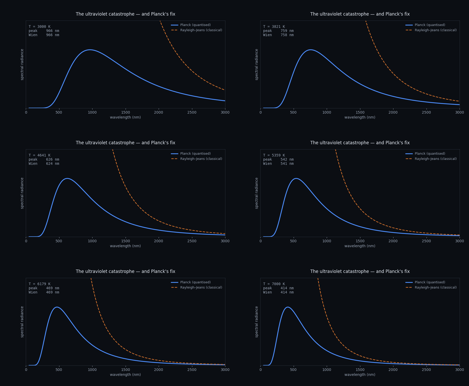
Classical physics predicted infinite energy at short wavelengths. Quantising energy was the only fix — and it started everything.
- Watch for
- The dashed classical curve shoots off the top of the chart. The quantised curve turns over and peaks.
- Checked
- The numerical peak matches Wien’s displacement law to within 0.3% across 3000–7000 K.
- Method
- Planck’s law evaluated directly against the Rayleigh–Jeans limit, SI constants.
Bohr’s atom and the hydrogen spectrum
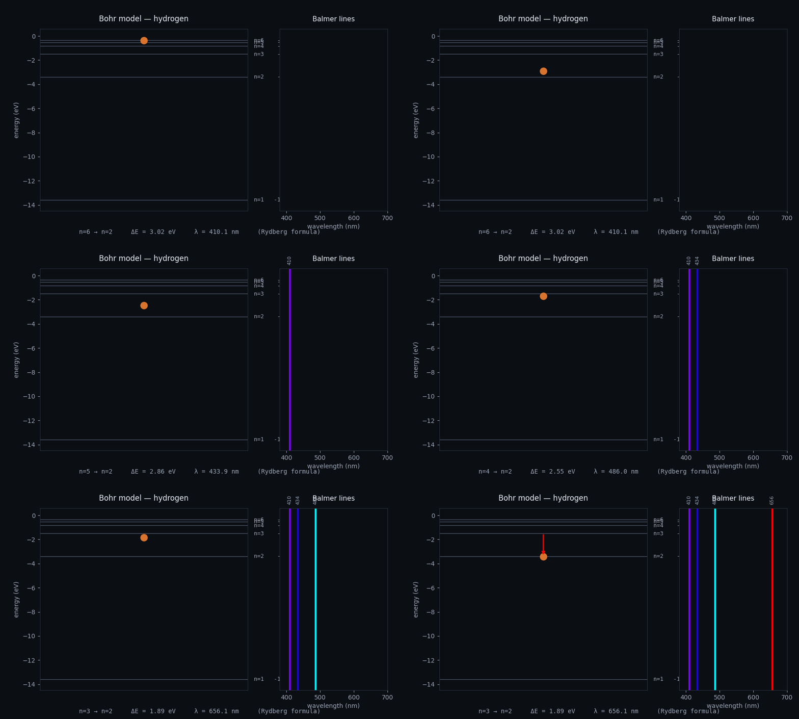
An electron drops between fixed levels and emits a photon. The four visible Balmer lines build up as it goes.
- Watch for
- Each drop emits one line at a specific colour. Bigger energy gaps give bluer light.
- Checked
- Wavelengths computed from the Rydberg formula land within 0.03% of the accepted Balmer values (656.11 vs 656.3 nm).
- Method
- Eₙ = −13.606/n² eV; wavelengths from the Rydberg formula; colours from the visible spectrum.
Born’s rule: probability from amplitude
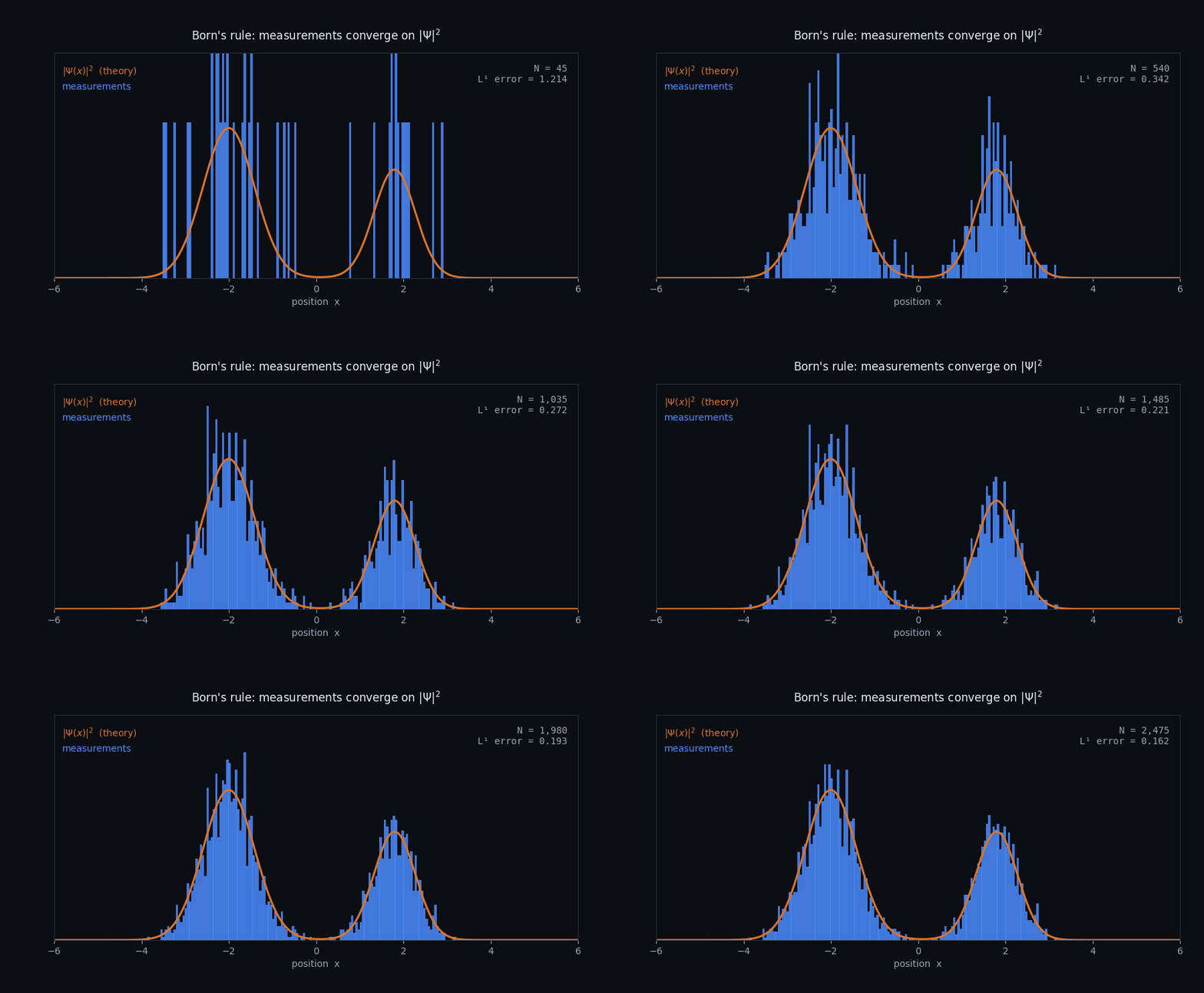
One measurement tells you almost nothing. Thousands reconstruct |Ψ|² exactly — which is all Ψ ever promised.
- Watch for
- The L¹ error between measurement and theory, printed live, falls as samples accumulate.
- Checked
- Error drops from 1.21 to 0.16 over 2,475 samples, converging monotonically on the true density.
- Method
- Sampling a two-peak |Ψ|², normalised identically to the theory curve for direct comparison.
Deriving the Schrödinger equation
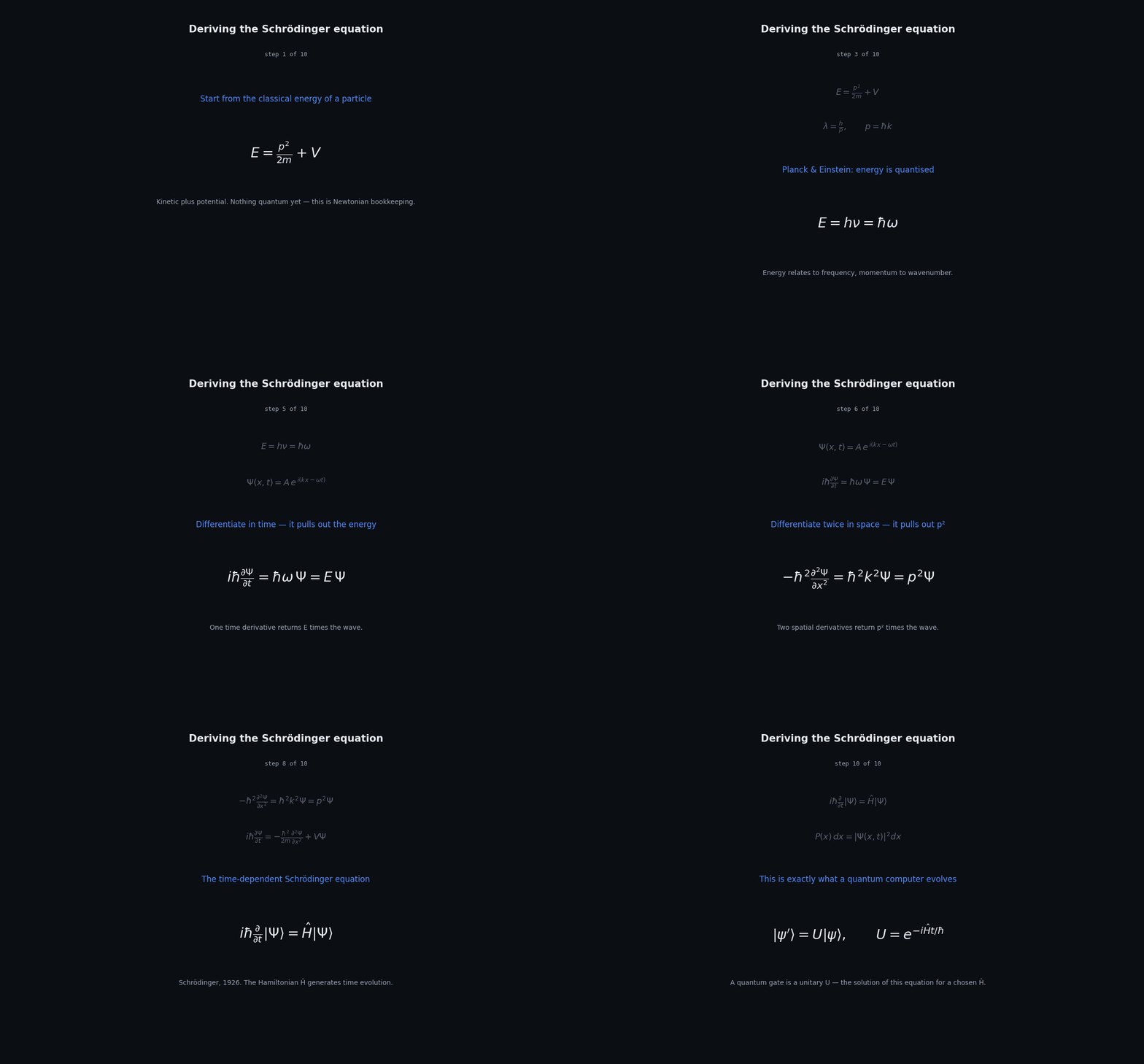
Ten steps from the classical energy of a particle to iℏ ∂Ψ/∂t = ĤΨ, and on to what a quantum gate actually is.
- Watch for
- Each step keeps the previous two on screen, so you can see the substitution that turns E and p² into operators.
- Checked
- Ends at U = e^(−iĤt/ℏ) — the unitary a quantum gate implements.
- Method
- Rendered from the derivation chain; each equation typeset from LaTeX.
Quantum tunnelling
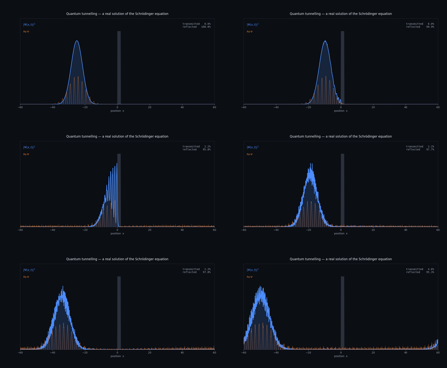
A wavepacket meets a barrier taller than its energy. Classically nothing gets through. Part of it does.
- Watch for
- The probability density splits at the barrier. The transmitted and reflected fractions are printed live.
- Checked
- Transmitted + reflected = 1.000 at every frame — probability is conserved. 4.6% tunnels through.
- Method
- Split-step Fourier integration of iℏ∂Ψ/∂t = ĤΨ, ħ = m = 1, 1024 grid points.
Heisenberg uncertainty in motion
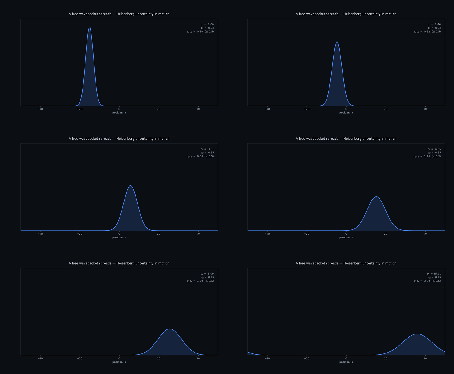
A free particle’s position spreads while its momentum spread stays fixed — the uncertainty product only grows.
- Watch for
- σₓ climbs frame by frame; σₖ does not move. Their product is printed on screen.
- Checked
- σₓ·σₖ starts at exactly 0.500 — a minimum-uncertainty Gaussian — and never drops below it.
- Method
- Same TDSE solver with V = 0; σₖ measured from the Fourier transform of Ψ.
Double slit, one detection at a time
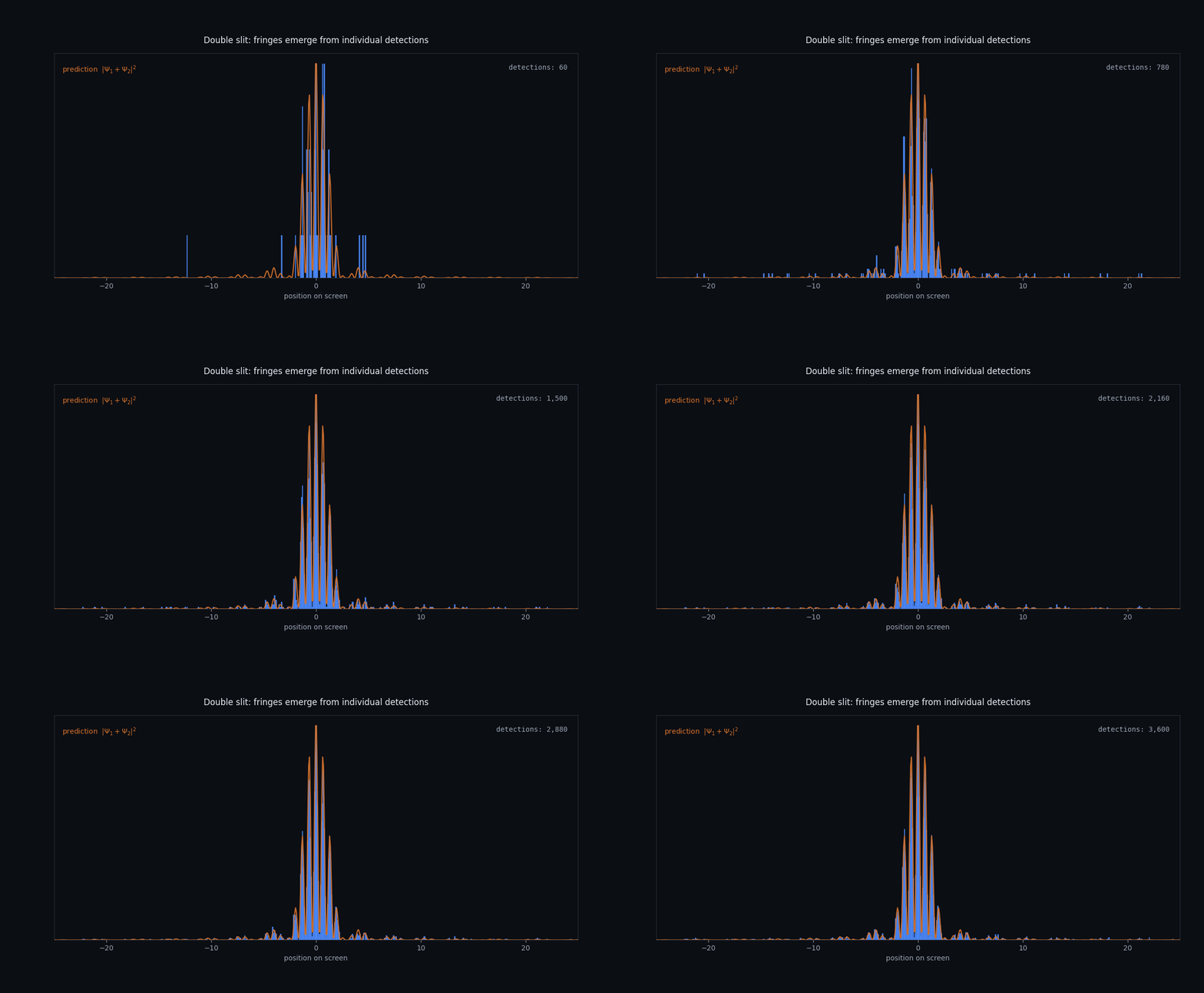
Each detection is a single dot. The fringes are not in any one of them — they emerge from thousands.
- Watch for
- The early frames look random. The predicted |Ψ₁+Ψ₂|² curve is overlaid so you can watch the data converge onto it.
- Checked
- Detections are sampled from the true two-slit intensity, including the single-slit envelope.
- Method
- Sampling from sinc²(β)·cos²(δ) — the exact two-slit intensity with finite slit width.
Phase precession on the Bloch sphere
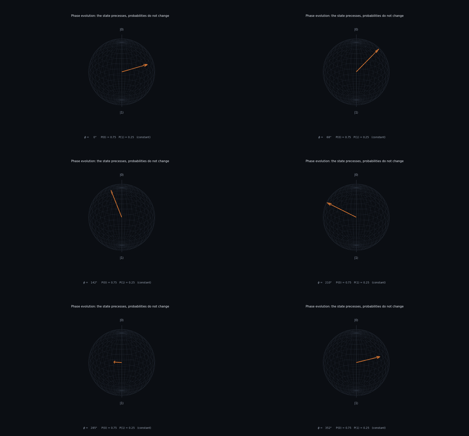
Phase evolution moves the state without changing any measurement probability in the computational basis.
- Watch for
- The arrow sweeps a full circle. P(0) and P(1) never budge — which is exactly why phase is invisible until you interfere.
- Checked
- Polar angle held fixed, so P(0) = cos²(θ/2) is constant by construction.
- Method
- Bloch vector traced at fixed θ with φ advancing through 2π.
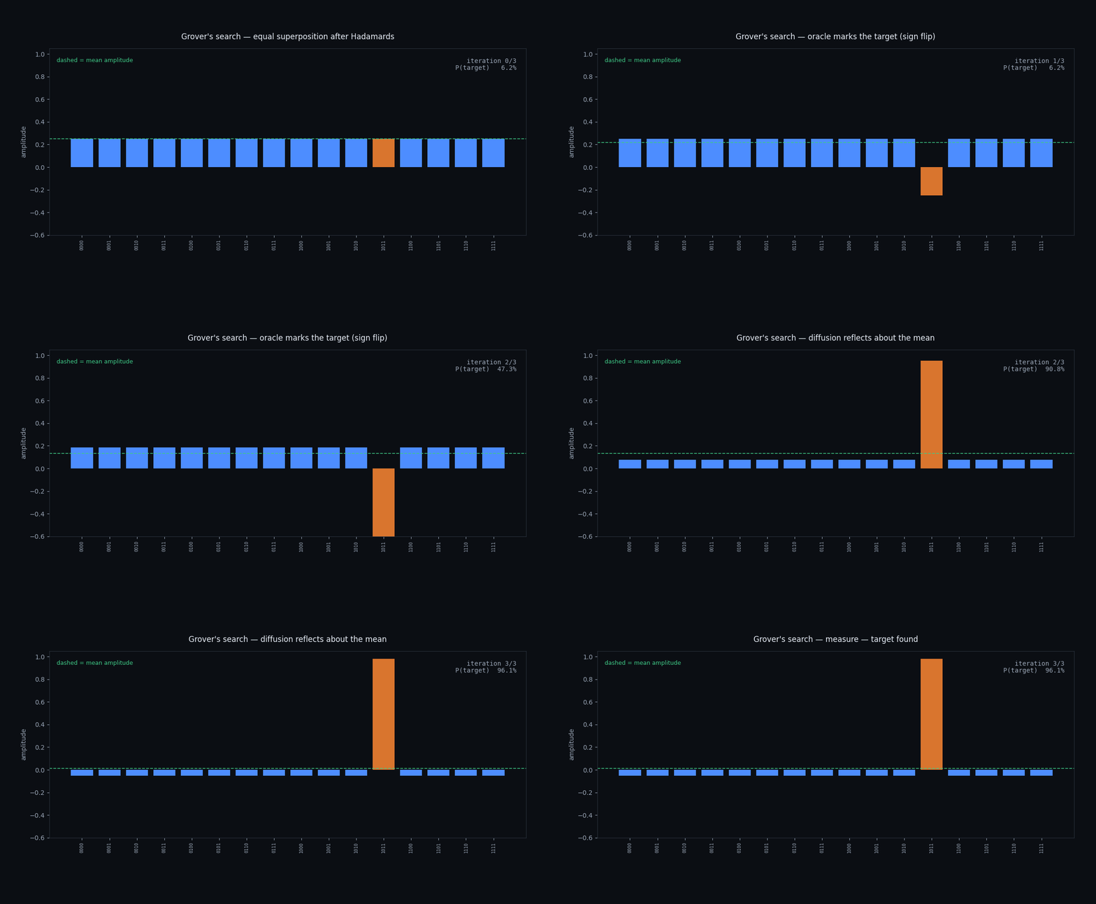
Grover: oracle and diffusion, step by step
Watch the two operations that make Grover work, on real amplitudes, one at a time.
- Watch for
- The oracle only flips a sign — the bar heights are unchanged. Diffusion does the amplifying, reflecting about the dashed mean.
- Checked
- P(target) goes 6.25% → 47% → 91% → 96%. 1/N = 6.25% for N = 16, and ⌈π/4·√16⌉ = 3 iterations.
- Method
- Real amplitude vector; oracle applies a sign flip, diffusion applies 2⟨a⟩ − a.
Regenerate at any resolution with python3 scripts/generate_physics_animations.py --width 1200